From raw forecast data to live CLOB orders, step by step.

Weather markets on Polymarket look deceptively simple. A city, a date, a temperature. But underneath that simplicity is a structure that rewards traders who understand numerical weather prediction and punishes those who don't. The edge isn't about being a better forecaster than the crowd. It's about being faster, more precise, and less wrong in predictable ways.
This guide walks through every layer of the stack: what these markets actually are, where the mispricing comes from, how to pull and correct forecast data for free, how to convert a model output into a probability distribution across buckets, and how to post orders through the CLOB API. Each section builds on the one before it. Follow them in order and you'll have a working foundation by the end.
One thing to set expectations on before you start: the edge in the most liquid markets has already compressed significantly, and it will keep compressing. That doesn't mean the opportunity is gone. It means the bot you build today needs to be faster and more precise than the one that worked two years ago. The sections below are written with that reality in mind.
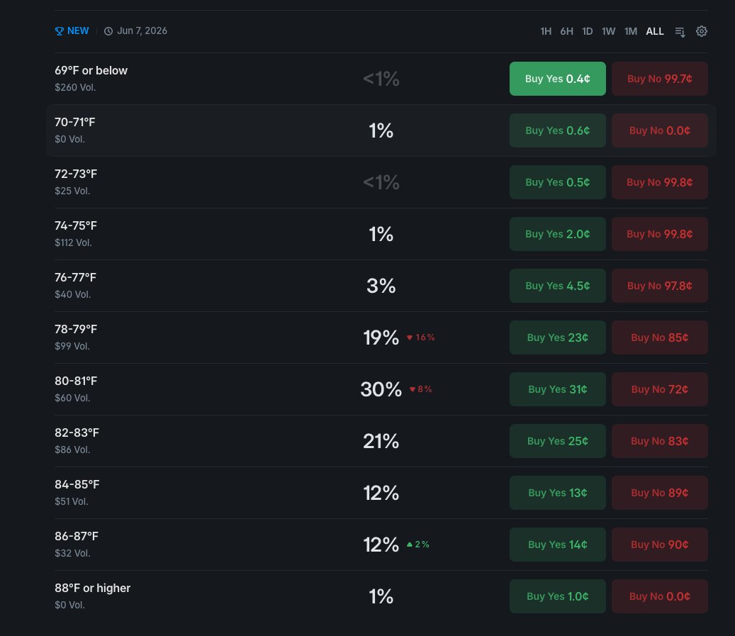
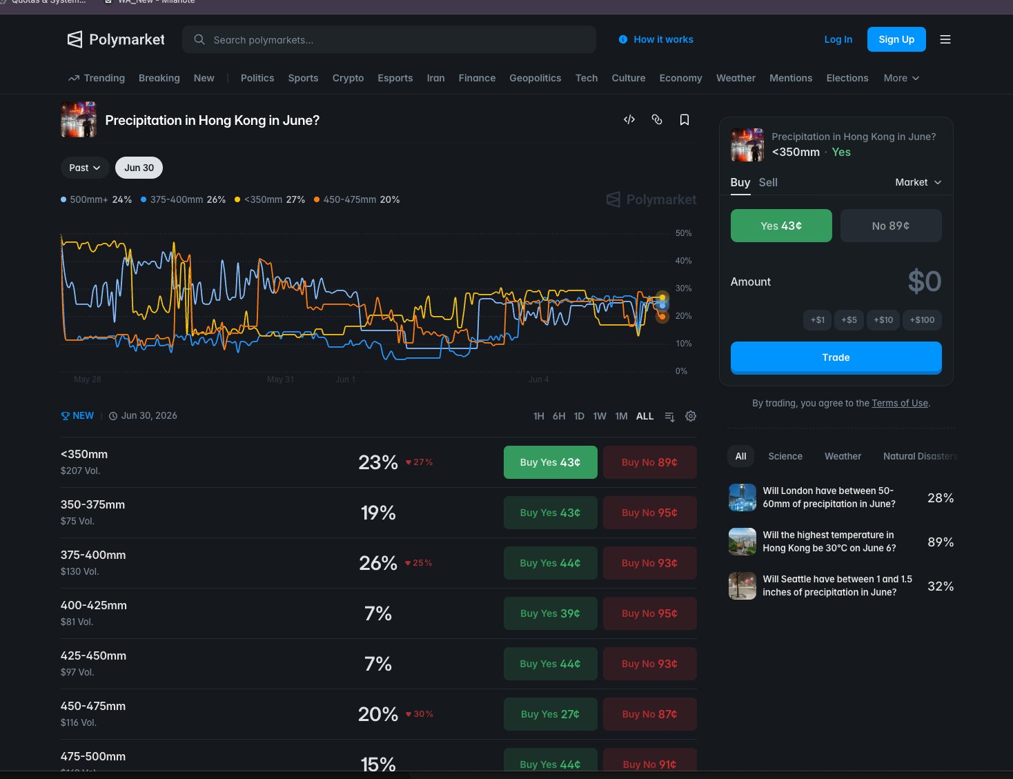
A Polymarket weather market is a single question about a single measurement at a single location on a single day. The answer gets split into a ladder of narrow price buckets, each trading independently. A price of 30 cents on a bucket means the market thinks there's roughly a 30% chance the day's high lands there.
Most people approach a weather market like a single bet. The pros treat it as a probability distribution spread across a row of adjacent contracts. That distinction changes everything about how you build a bot to trade them.
The most common form is 'Highest temperature in [city] on [date]?' and the resolution space gets carved into mutually exclusive buckets, each priced from 0 to 100 cents. Exactly one bucket resolves YES, so the prices across all buckets in a market should sum to roughly 100 cents. That's not a coincidence or a convention. It's a hard structural constraint, and it's the first thing your bot should verify on every book snapshot.
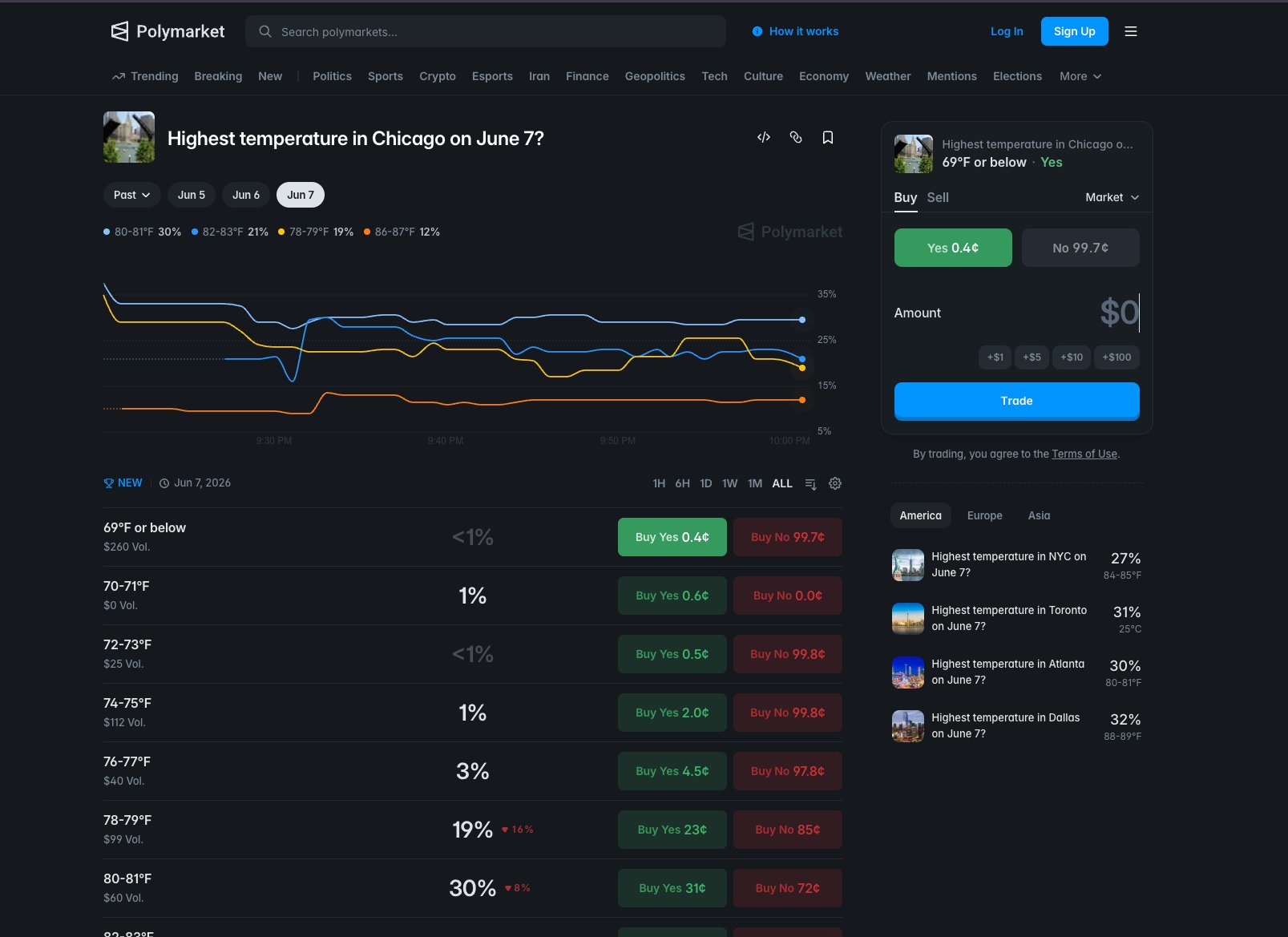
That 2°F width is the critical structural fact to internalize before writing a single line of code. A weather model with a mean absolute error of 1.5°F sounds accurate in isolation. Inside a 2°F bucket, that same error is enough to push your probability mass into the wrong contract on a regular basis. You're not forecasting temperature. You're forecasting which specific 2°F slice temperature lands in. Those are different problems.
Each bucket trades as a separate instrument with its own token_id, its own order book, and its own bid-ask spread. You can be long one bucket and short its immediate neighbor at the same time. The market doesn't enforce any relationship between adjacent bucket prices. That's your job.
token_id and independent order book.Don't assume every weather market trades the same. A busy NYC daily-high market can clear six figures of volume in a single day. A quieter secondary city might do a fraction of that. Thin books mean wider spreads and more slippage, which changes the edge threshold you need before placing an order. Build city-level liquidity tracking into your data model from day one, not as an afterthought.
observed Sum-to-100 divergence in a scraped book snapshot is a reliable signal of a stale or malformed response. Re-fetch before acting.
Your bot needs to track every bucket in a market as a separate tradeable instrument, not just the most likely outcome. Store each bucket's token_id, price range, current best bid, and best ask as distinct rows in your data model. When your probability model produces a vector of probabilities across all buckets, compare each bucket's model probability against its current market price independently. Use the sum-to-100 constraint as a consistency check on every book snapshot: if the prices you scraped sum to significantly more or less than 100 cents, you have a stale or malformed response and should re-fetch before placing any orders.
# Pseudocode: validate a market snapshot before use

def validate_bucket_snapshot(buckets: list[dict]) -> bool:
    """
    buckets: list of dicts, each with keys:
        token_id  (str)
        label     (str, e.g. '88-90°F')
        best_bid  (float, cents)
        best_ask  (float, cents)
        mid       (float, cents)  # (best_bid + best_ask) / 2
    """
    total_mid = sum(b['mid'] for b in buckets)

    TOLERANCE = 5.0  # cents, adjust based on observed spread width

    if abs(total_mid - 100.0) > TOLERANCE:
        # Snapshot is stale or malformed. Do not trade.
        return False

    return True

# If validate_bucket_snapshot returns False, re-fetch the order book.
# Never place an order against a snapshot that fails this check.The edge in weather markets isn't about predicting the weather better than everyone else. It's about reading the same free data faster than the crowd does. Professional weather models publish new forecasts on a fixed schedule, and the market is slow to catch up every single time.
Most people assume you need a proprietary forecast to beat a prediction market. Actually, the pros aren't building better models than ECMWF or NOAA. They're just reading ECMWF and NOAA output before the crowd does, and acting on the gap before it closes.
The three major numerical weather prediction models, ECMWF IFS, NOAA GFS, and the GEFS ensemble, run on fixed six-hour cycles at 00Z, 06Z, 12Z, and 18Z. Each completed run produces a revised predicted daily maximum. When that revision is large enough to shift a bucket's fair value, the market should reprice immediately. It doesn't, because retail participants are reading weather apps and news articles, not raw model output feeds. That lag is the window.
Not all markets reprice at the same speed. The mispricing window splits cleanly along liquidity lines, and that split should drive every architectural decision you make.
Mispricing window of roughly 5 to 15 minutes after a new model run lands. Already compressed from a 30 to 60 minute window as recently as 2024. Requires a tight, low-latency pipeline. Margin for error is small.
Mispricing window measured in hours, not minutes. The crowd takes hours to reprice what the model already published. A slower, cheaper polling loop still captures the full gap.
observed NYC and London have compressed from a 30 to 60 minute window in 2024 down to roughly 5 to 15 minutes today. That compression is ongoing, not a one-time event.
That asymmetry is structural, not accidental. Liquid markets attract more sophisticated participants who have already built faster pipelines. Secondary markets haven't hit that threshold yet. Build your architecture around which market you're targeting first, because the latency requirement for NYC is an order of magnitude tighter than for Seoul.
A new model run doesn't always move the needle. The signal you care about is a revision large enough to shift a bucket's fair value past your edge threshold. Think of it like a price-to-value gap in equities: you don't act on every tick, only when the discount is wide enough to cover your costs and still leave profit. In weather markets, that threshold is a function of how much the new model run moved the predicted temperature and how that movement maps to bucket probabilities.
Build your entry trigger around model-run detection, not a fixed polling interval. Cache each API response keyed to its update timestamp. When a new run arrives and your probability model shifts a bucket's fair value past your edge threshold (start at 8%, then tune from your own backtest), that's your signal to act. Subscribe to the CLOB WebSocket for book and price_change events so you know the moment the crowd starts repricing, and pull any resting passive orders before the edge closes. On NYC and London you have 5 to 15 minutes. On Seoul, Wellington, and Moscow the window stretches hours, so a slower polling loop is still profitable there.
# Pseudocode: model-run detection trigger

last_seen_run_timestamp = cache.get('last_model_run_ts')

current_run = fetch_latest_model_output(city='NYC', model='GFS')

if current_run.timestamp != last_seen_run_timestamp:
    cache.set('last_model_run_ts', current_run.timestamp)

    new_fair_values = compute_bucket_probabilities(current_run.predicted_max_temp)
    prev_fair_values = cache.get('last_fair_values')

    for bucket in open_buckets:
        shift = abs(new_fair_values[bucket] - prev_fair_values[bucket])
        if shift >= EDGE_THRESHOLD:   # start at 0.08, tune from backtest
            signal_queue.push({
                'bucket': bucket,
                'direction': 'buy' if new_fair_values[bucket] > market_price[bucket] else 'sell',
                'fair_value': new_fair_values[bucket],
                'market_price': market_price[bucket],
                'shift': shift
            })

    cache.set('last_fair_values', new_fair_values)
Every Polymarket weather market resolves against one specific physical weather station, not a general city location. If you query the wrong coordinates, your forecast can be off by 3 to 8 degrees Fahrenheit on markets where the winning bucket is only 1 to 2 degrees wide. That doesn't shrink your edge, it flips your bets to the wrong side on boundary trades.
Most people building weather bots pull forecast data for a city name or a city-center coordinate. The pros parse the station code out of the market's Rules text before touching any forecast API. The difference isn't academic. A 3 to 8°F offset between a city-center point and an airport station is a consistent directional bias, not noise, and it's driven by three compounding factors: the urban heat-island effect, elevation differences, and proximity to water.
Take New York City as a concrete example. LaGuardia (KLGA) sits on a peninsula in Flushing Bay. Central Park (KNYC) sits inside a concrete grid. Neither matches a midtown rooftop sensor, and Polymarket has cited both across different resolution dates. You cannot hardcode one. If you lock in KLGA and Polymarket resolves against KNYC that week, you've introduced a systematic offset before your model has even run.
observed Polymarket has cited both KLGA and KNYC for New York City across different resolution dates. Parse the station from the Rules text on every cycle.
Convenient to hardcode. Introduces 3 to 8°F systematic bias. Matches no resolution source. Confidently wrong on boundary trades.
Requires a fresh parse each cycle. Zero systematic offset. Matches the exact source Polymarket uses. Correct on boundary trades.
The right implementation is a registry keyed by ICAO code. Each entry stores exact lat/lon, data provider, unit system, and reported precision. Precision belongs on the station record, not as a global setting, because HKO's 0.1°C resolution means boundary buckets are priced differently than they would be under whole-degree rounding at a US station.
STATION_REGISTRY = {
  "KLGA": {
    "lat": 40.7772,
    "lon": -73.8726,
    "provider": "nws",          # api.weather.gov/points/{lat},{lon}
    "unit": "fahrenheit",
    "precision": 1.0            # whole degrees
  },
  "KNYC": {
    "lat": 40.7789,
    "lon": -73.9692,
    "provider": "nws",
    "unit": "fahrenheit",
    "precision": 1.0
  },
  "RKSI": {
    "lat": 37.4691,
    "lon": 126.4505,
    "provider": "open_meteo",
    "unit": "celsius",
    "precision": 1.0
  },
  "HKO": {
    "lat": 22.3020,
    "lon": 114.1740,
    "provider": "hko_direct",   # separate query path, not on standard aggregators
    "unit": "celsius",
    "precision": 0.1            # 0.1°C resolution changes bucket boundaries
  }
}

def get_station_for_market(market_rules_text: str) -> dict:
    """Parse ICAO code from Rules text. Return registry entry.
       Raise UnresolvableMarket if code not found in registry."""
    icao = extract_icao_from_rules(market_rules_text)  # regex over known codes
    if icao not in STATION_REGISTRY:
        raise UnresolvableMarket(f"Unknown station: {icao}. Review manually.")
    return STATION_REGISTRY[icao]
For US stations, the NWS api.weather.gov/points/{lat},{lon} endpoint resolves coordinates to the correct forecast gridpoint and also exposes hourly station observations. That gives you forecast and historical actuals from one pipeline. For international stations, use published ICAO coordinates with Open-Meteo. For Hong Kong, build a separate HKO query path entirely. HKO data isn't on Weather Underground or any standard aggregator.
In your discovery loop, extract the station code from each market's Rules text on every cycle before touching any forecast API. If your parser can't find a known ICAO code in the registry, treat the market as unresolvable and skip it until you've checked manually. Never cache a city-level coordinate. One mismatched station on a boundary trade costs more than a dozen correct trades earn back. Store precision per station in the registry, not globally, because HKO's 0.1°C resolution means every boundary bucket is priced differently than it would be under whole-degree rounding.
You don't need to pay for weather data to build a working bot. Open-Meteo, the National Weather Service, and NOAA between them cover every forecast and historical observation you need. Paid services add convenience, not the difference between a profitable system and an unprofitable one.
Most people assume serious quantitative work requires expensive data subscriptions. The free stack here is genuinely complete: ensemble probabilities, intraday station observations, and decades of archive-grade ground truth, all without a single invoice.
Open-Meteo aggregates more than 30 numerical weather models, including ECMWF IFS, NOAA GFS and HRRR, DWD ICON, and the 31-member GEFS ensemble. It processes over 2 TB of data daily from national weather services worldwide, requires no API key or account, and is free for non-commercial use under CC-BY 4.0. That's a serious data pipeline, not a hobbyist project.
Rate limits are tiered at 10,000 calls per day, 5,000 per hour, and 600 per minute. For a bot tracking roughly 20 active market groups with hourly polling, that ceiling is comfortable. You'd have to work hard to hit it.
There's a critical difference between what the model predicted on a past date and what actually happened. Most people only pull observed outcomes. That's the wrong dataset for bias-correction training.
observed Open-Meteo's Historical Forecast API covers data from roughly 2021 onward and returns what the model predicted on a specific past date, not the verified observation. Pair those archived predictions against NOAA GHCN-Daily actuals and you have a ready-made bias-correction training set.
Open-Meteo: ensemble forecast probabilities, historical model predictions back to ~2021, global coverage, no auth. NWS api.weather.gov: official US gridpoint forecasts and intraday hourly station observations (KLGA, KNYC, etc.), User-Agent header only. NOAA GHCN-Daily: decades of TMAX, TMIN, and PRCP with a 45–60 day lag, archive-grade ground truth.
Open-Meteo: primary forecast engine and bias-correction training data. NWS: intraday convergence logic and end-of-day observation reads. NOAA GHCN-Daily: calibration archive, not a live feed. Use it to validate your bias-correction model, not to make same-day decisions.
NWS only requires a User-Agent header in your requests, which is a one-line addition to any HTTP client. NOAA GHCN-Daily is a flat-file archive you can download once and update incrementally. Neither requires registration.
# Open-Meteo: pull all 31 GEFS ensemble members for a specific station
import openmeteo_requests

om = openmeteo_requests.Client()

params = {
    "latitude": 40.7769,       # KLGA exact coords, not Midtown
    "longitude": -73.8740,
    "models": "gefs025",       # 31-member ensemble
    "hourly": ["temperature_2m"],
    "forecast_days": 7
}

response = om.weather_api("https://ensemble-api.open-meteo.com/v1/ensemble", params=params)

# Historical Forecast API: what did the model predict on 2024-01-15?
hist_params = {
    "latitude": 40.7769,
    "longitude": -73.8740,
    "models": "gfs_seamless",
    "hourly": ["temperature_2m"],
    "start_date": "2024-01-15",
    "end_date": "2024-01-15"
}

hist_response = om.weather_api(
    "https://historical-forecast-api.open-meteo.com/v1/forecast",
    params=hist_params
)

# NWS: intraday station observations (User-Agent header required)
import requests

headers = {"User-Agent": "your-bot-name contact@youremail.com"}
obs_url = "https://api.weather.gov/stations/KLGA/observations/latest"
nws_obs = requests.get(obs_url, headers=headers).json()
Query Open-Meteo at the exact station coordinates from your market registry, not the city center. KLGA is at 40.7769, -73.8740, not Midtown Manhattan. Use the gefs025 model parameter to pull all 31 ensemble members and compute your own probability distribution across them. For bias-correction training, pull the Historical Forecast API for each station going back to 2021, then pair those archived model predictions against GHCN-Daily actuals. For US markets, pipe NWS api.weather.gov hourly observations into your end-of-day convergence logic: your bot should be reading the same source Polymarket's resolution oracle reads. If a backtest on this free stack doesn't show positive EV, paying for a premium feed won't fix it. Spend on paid data only after the edge is proven.
A weather model gives you one number: its best guess at the day's high temperature. That single number is useless for betting on a bucket. You need to know the probability that the actual high lands inside a specific 2°F range, which means turning that point estimate into a spread of likelihoods across every bucket on the ladder.
Most people look at a model forecast and think the number is the answer. It isn't. A forecast of 91°F tells you nothing about whether the actual high lands in the 90–92°F bucket versus the 88–90°F bucket. The pros treat that forecast as the center of a distribution, then ask: given how wrong this model typically is at this lead time, at this station, in this season, what fraction of that distribution falls inside each bucket?
Apply your bias correction first (Step 04), then treat the corrected forecast as the mean of a normal distribution. The standard deviation comes from your own historical error analysis, fit by station, lead time, and season. Illustrative starting values run from roughly 0.8°F at a 6-hour lead to around 5.5°F at 10 days. Bucket probability is the integral of the normal CDF between the bucket's lower and upper bounds.
from scipy.stats import norm

def bucket_probs_gaussian(mu, sigma, buckets):
    """
    mu     : bias-corrected forecast (°F)
    sigma  : station/lead/season error std (°F)
    buckets: list of (lower, upper) tuples
    returns: probability vector summing to 1.0
    """
    probs = []
    for lower, upper in buckets:
        p = norm.cdf((upper - mu) / sigma) - norm.cdf((lower - mu) / sigma)
        probs.append(p)
    total = sum(probs)
    return [p / total for p in probs]  # renormalize to handle open-ended tails
With ensemble output, skip the Gaussian entirely. Each of the 31 GEFS members is an independent draw from the model's uncertainty space, so you already have an empirical distribution. Count how many members land inside each bucket, divide by 31, then optionally smooth with a light Gaussian filter to reduce discretization noise at small N.
import numpy as np
from scipy.ndimage import gaussian_filter1d

def bucket_probs_ensemble(members, buckets, smooth_sigma=0.8):
    """
    members: array of 31 temperature forecasts (°F)
    buckets: list of (lower, upper) tuples
    returns: probability vector summing to 1.0
    """
    counts = np.array([
        np.sum((members >= lo) & (members < hi))
        for lo, hi in buckets
    ], dtype=float)
    if smooth_sigma > 0:
        counts = gaussian_filter1d(counts, sigma=smooth_sigma)
    total = counts.sum()
    return counts / total if total > 0 else counts
After producing both vectors, blend by skill weight. The deterministic run tends to outperform the ensemble mean inside 48 hours. Beyond 5 days, the ensemble spread is the more reliable signal. Once blended, apply a final pull toward the 10-year climatological base rate for that calendar date at that station. This keeps extreme estimates honest when the model is running unusually hot or cold.
def blend_and_anchor(det_probs, ens_probs, det_weight, climo_probs, climo_weight=0.08):
    """
    det_weight : scalar 0.0–1.0 (higher inside 48 h, lower beyond 5 days)
    climo_weight: fraction pulled toward climatology (start at 0.08)
    """
    ens_weight = 1.0 - det_weight
    blended = [
        det_weight * d + ens_weight * e
        for d, e in zip(det_probs, ens_probs)
    ]
    anchored = [
        (1 - climo_weight) * b + climo_weight * c
        for b, c in zip(blended, climo_probs)
    ]
    total = sum(anchored)
    return [p / total for p in anchored]  # final renormalize
Lean on the deterministic run. Bias-corrected GFS or ECMWF single-model output has lower RMSE at short leads. Set det_weight to 0.7–0.8 and let the ensemble fill the rest.
Flip the weights. Ensemble spread captures uncertainty the deterministic run can't express at long leads. Set det_weight to 0.2–0.3 and let the 31-member spread dominate.
observed The output of this step is a single probability vector summing to 1.0 across all buckets. Subtract market prices from that vector and you have your raw edge before any position sizing.
Each bucket in a Polymarket temperature market has its own YES/NO price. Your probability vector maps directly onto those prices. If your model assigns 0.42 to the 88–90°F bucket and the market is offering YES at 0.31, that's an 11-cent edge on the YES side before spread. Run this calculation across every bucket after each new model run at 00Z, 06Z, 12Z, or 18Z. Flag any bucket where the absolute difference between your probability and the best ask (for YES) or best bid (for NO) clears your minimum threshold, starting at 8%. Use the ensemble member-count path when querying Open-Meteo with models='gefs025', which returns all 31 GEFS members. Fall back to the Gaussian path when only a deterministic GFS or ECMWF run is available. The climatological anchor matters most on Polymarket because extreme model runs attract attention and push market prices to their own extremes. Pulling your estimate back toward the base rate keeps you from chasing a mispriced crowd in the wrong direction.
Weather models are wrong in predictable ways, and you can measure and remove most of that error before you ever touch machine learning. Three classical methods handle the bulk of it: exponential smoothing, Model Output Statistics, and a Kalman filter. Each one is simple to implement and hard to overfit.
Most new bot builders skip straight to XGBoost or a U-Net and wonder why the system that looked sharp in a notebook loses money live. The pros do something different: they remove the predictable, systematic error first, using methods that have been battle-tested in operational meteorology for decades, and only then layer on anything fancier. These three methods together remove 60–80% of achievable systematic bias before a single ML weight is trained.
The core problem is that a GFS grid cell near LaGuardia is not LaGuardia. The model's 2-meter temperature carries systematic bias that shifts by location, season, and lead time. That bias is not random noise. It's structured, it's measurable, and it compounds directly into bad bucket probabilities if you leave it in.
This is the fastest to implement and the most common starting point. You track the model's recent errors and fade out the influence of older ones using a decay parameter alpha. Set alpha between 0.95 and 0.98. Higher alpha means older errors stay relevant longer, which is right for slow-moving seasonal drift. Lower alpha lets the corrector react faster to abrupt shifts. The compute cost is essentially zero: one multiply and one add per observation.
# Exponential smoothing bias corrector
# bias_t: current bias estimate
# error_t: (observed - forecast) at time t
# alpha: smoothing factor, typically 0.95–0.98

bias_t1 = alpha * bias_t + (1 - alpha) * error_t
corrected_forecast = raw_forecast + bias_t1
observed Alpha in the 0.95–0.98 range captures seasonal and regional bias effectively at near-zero compute cost. Values outside this range tend to either overreact to single outliers or adapt too slowly to real drift.
MOS is a meteorology classic that still outperforms most ML approaches on small datasets. You fit a simple linear regression to the raw forecast, using the model output as your predictor and observed surface measurements as your target. The real power comes from adding covariates: cloud cover, wind speed, land type, and elevation all help the regression absorb the diurnal cycle that raw grid output consistently gets wrong. MOS requires a training set, but that's exactly what Open-Meteo's Historical Forecast API provides from roughly 2021 onward.
# MOS: fit a linear corrector per station per lead time
# Features: raw_temp, cloud_cover, wind_speed, land_type_encoded
# Target: observed_temp

from sklearn.linear_model import LinearRegression

X_train = historical_forecasts[['raw_temp', 'cloud_cover', 'wind_speed', 'land_type']]
y_train = historical_observations['observed_temp']

mos_model = LinearRegression().fit(X_train, y_train)
corrected_forecast = mos_model.predict(X_live)
The Kalman filter is the most adaptive of the three. Instead of fitting a static corrector, it updates the bias estimate continuously in real time, scaling the correction by how much trust the model has recently earned. When the model has been accurate, the filter leans on its own prior estimate. When recent errors are large, it weights new observations more heavily. This makes it the right choice when you're tracking multiple cities or when GFS or ECMWF pushes a version update that shifts the model's baseline.
# Simplified scalar Kalman filter for bias tracking
# bias: current bias estimate
# P: estimate uncertainty
# Q: process noise (how fast bias drifts)
# R: observation noise (sensor/measurement uncertainty)

K = P / (P + R)                        # Kalman gain
bias = bias + K * (observed - (forecast + bias))  # update
P = (1 - K) * P + Q                    # update uncertainty
observed The Kalman filter adapts cleanly to season transitions and model version updates without requiring a full refit. That's a meaningful operational advantage over static MOS when you're running markets across many cities simultaneously.
The model looks precise in backtests because it memorizes historical noise. Live, it encounters the same systematic bias the raw forecast always had, and the ML layer has no mechanism to separate that from signal. Losses accumulate in a pattern that's hard to diagnose.
The corrector removes 60–80% of systematic error with near-zero overfitting risk. Any ML layer added afterward is working on residuals that are much closer to true noise, so it has a realistic chance of finding genuine signal rather than chasing structured error.
Run one of these three correctors on every forecast before you compute bucket probabilities. Exponential smoothing is the fastest to wire in: store a running bias estimate per station and update it after each resolved market. MOS requires a training set, which Open-Meteo's Historical Forecast API provides from roughly 2021 onward. The Kalman filter is the right choice once you're tracking multiple cities and want the bias estimate to adapt automatically when a GFS or ECMWF version update shifts the model's baseline. Whichever method you choose, apply it before the Gaussian or ensemble bucket-probability step from Step 05. Skipping bias correction and going straight to ML is the most common way new bot builders produce a system that looks sharp in a notebook and loses money live.
Once your model spits out a probability for each bucket, compare it to what the market is actually charging. If the gap isn't wide enough to cover the spread, fees, and the natural randomness of weather forecasts, you don't trade. A 2-point edge isn't a trade, it's noise.
Most people think edge means being right more often than the market. It doesn't. Edge means being right by enough to overcome the spread, fees, and the irreducible variance baked into short-range forecasts. A model reading of 55% against a market ask of 53% looks like an edge. It isn't. That 2-point gap evaporates the moment you account for the bid-ask spread and the fee on settlement.
The minimum edge practitioners cite to stay profitable is 8%, measured simply: model_prob - best_ask for a YES trade, or best_bid - model_prob for a NO trade. Treat 8% as a calibration starting point, not gospel. Your own backtest across your specific cities and forecast horizons may tell you 6% or 10% is the right floor. But start at 8% and let the data move you.
def compute_edge(model_prob, best_ask, best_bid):
    edge_yes = model_prob - best_ask      # positive = YES has edge
    edge_no  = (1 - model_prob) - (1 - best_bid)  # equiv: best_bid - model_prob
    return edge_yes, edge_no

MIN_EDGE = 0.08

edge_yes, edge_no = compute_edge(model_prob=0.55, best_ask=0.53, best_bid=0.50)
# edge_yes = 0.02  -> below threshold, no trade
# edge_no  = -0.05 -> no edge on NO side either
Full Kelly is mathematically optimal and practically brutal. One bad streak puts you down 40% before you've had time to diagnose whether the model is broken or just unlucky. The fix is quarter-Kelly with a hard 5% per-market cap. The 5% cap is a ceiling, not a target. Quarter-Kelly keeps you solvent long enough for the edge to compound across hundreds of trades.
def kelly_size(edge, odds, bankroll, kelly_fraction=0.25, max_pct=0.05):
    # edge = model_prob - price paid
    # odds = (1 / price) - 1  (net odds on a binary)
    full_kelly = edge / odds
    fractional = full_kelly * kelly_fraction
    capped = min(fractional, max_pct)
    return capped * bankroll

# Example: edge=0.12, price=0.40, bankroll=$10,000
# full_kelly = 0.12 / 1.50 = 0.080
# quarter_kelly = 0.020  -> $200
# cap check: 2.0% < 5.0% -> position = $200
Mathematically maximizes long-run growth. In practice, a 5-loss streak at full Kelly can draw down 40%+ and force you to recalibrate under pressure, when you're least objective.
Grows more slowly but survives bad streaks. Position sizes shrink automatically as bankroll drops. The 5% cap prevents any single market from doing serious damage.
Trading 20+ markets beats concentrating in 2, but only if those markets are genuinely independent. Weather is regionally correlated: a single cold snap can simultaneously hit Chicago, NYC, and Boston. If your bot fires full-size entries across all three at once, you've accidentally concentrated your risk. Apply a correlation haircut to your Kelly fraction for cities in the same climate zone.
REGIONAL_GROUPS = {
    'northeast_us': ['NYC', 'Boston', 'Philadelphia'],
    'midwest_us':   ['Chicago', 'Detroit', 'Cleveland'],
    'southeast_us': ['Atlanta', 'Miami', 'Charlotte'],
}

CORRELATION_HAIRCUT = 0.6  # reduce Kelly by 40% for same-region co-entries

def adjusted_kelly(city, active_positions, base_kelly):
    region = get_region(city)
    same_region_open = sum(
        1 for c in active_positions if get_region(c) == region
    )
    haircut = CORRELATION_HAIRCUT ** same_region_open
    return base_kelly * haircut
Brier score measures calibration on a 0.0 to 0.25 scale. A perfectly calibrated model scores 0.0. Random 50/50 guessing scores 0.25. Track it per city and per forecast horizon on a rolling 30-day window. If a city's rolling Brier drifts above 0.15, flag it. Above 0.20, soft-disable it until you've diagnosed the cause. Don't wait for a catastrophic blowup to notice the model has gone stale.
(model_prob - outcome)^2, averaged over all resolved markets in the window.observed The 8% edge floor and the Brier soft-disable thresholds (0.15 flag, 0.20 disable) are figures practitioners have converged on through live trading, not theory. Your own calibration may shift them, but they're the right starting defaults.
In your bot's decision loop, compute edge_yes and edge_no after every model-run update and gate all order submission behind the 8% threshold. Wire kelly_size to your live bankroll tracker so position sizes shrink automatically during drawdowns. Store per-city Brier scores in a rolling database table (keyed by city + horizon) and add a pre-trade check that reads the soft-disable flag before submitting any order. When building out to 20+ markets, group cities by region in a config file and apply the correlation haircut to your Kelly fraction whenever two or more cities in the same group already have open positions. This prevents a single weather system from triggering simultaneous full-size entries across your entire northeast or midwest cluster.
Posting orders to Polymarket means talking to a central limit order book running on the Polygon blockchain. The py-clob-client library handles authentication, signing, and submission so you don't have to build any of that plumbing yourself. Once you're set up, you can post single orders, batch up to 15 at once, and subscribe to a WebSocket feed that delivers book updates roughly 10 times faster than polling REST.
Install the library with pip install py-clob-client. The stable production line is v0.34.6. An early-stage v2 exists but isn't production-ready for a bot that needs to run unattended.
Instantiate ClobClient with three things: chain_id=137 (Polygon mainnet), your private key, and a signature_type. Use 0 for a standard EOA wallet, 1 for a Magic or email-proxy wallet, and 2 for a Safe or browser-proxy wallet. Most bots use 0. Pass your funder address as well. Then call create_or_derive_api_creds() once to generate session credentials. Do this before anything else, and set token allowances before your first order or the submission will fail silently with no useful error.
from py_clob_client.client import ClobClient
from py_clob_client.clob_types import OrderArgs, OrderType

client = ClobClient(
    host="https://clob.polymarket.com",
    key=PRIVATE_KEY,
    chain_id=137,
    signature_type=0,
    funder=FUNDER_ADDRESS,
)

# Run once to generate session creds
client.create_or_derive_api_creds()

# Set allowances before first order
client.set_allowances()
Build an OrderArgs object with token_id, price, size, and side. Sign it with create_order(), then submit via post_order() with OrderType.GTC for a resting limit. When you want an immediate fill, post one tick through the best ask instead of switching order types. That said, the CLOB does support true market orders via FOK and FAK on MarketOrderArgs. Most weather plays use limits, but knowing FOK and FAK exist matters when your edge is time-sensitive.
from py_clob_client.clob_types import OrderArgs, OrderType, Side

args = OrderArgs(
    token_id=TOKEN_ID,
    price=0.61,
    size=50.0,
    side=Side.BUY,
)

signed_order = client.create_order(args)
resp = client.post_order(signed_order, OrderType.GTC)
print(resp)
When your model flags several mispriced buckets in the same market simultaneously, don't submit them one at a time. Sign each with create_order(), collect the signed objects into a list, and fire them all in a single post_orders() call. The batch cap is 15 orders per call. If you're trading more than 15 buckets at once, split into sequential batches and handle partial failures per batch before moving to the next.
signed_orders = []
for bucket in mispriced_buckets:          # up to 15
    args = OrderArgs(
        token_id=bucket["token_id"],
        price=bucket["edge_price"],
        size=bucket["size"],
        side=Side.BUY,
    )
    signed_orders.append(client.create_order(args))

# All orders hit the book in the same state
resp = client.post_orders(signed_orders)

# Handle partial failures before next batch
for result in resp:
    if result.get("status") != "matched" and result.get("status") != "live":
        log_failed_order(result)
observed Batching keeps all legs in the same book state. Submitting them sequentially means the first fill can move the market before the second order lands.
Polling REST is fine during development. In production it's too slow. Subscribe to wss://ws-subscriptions-clob.polymarket.com/ws/market instead. Use the book channel for full snapshots on connect, price_change for incremental updates as the book moves, and last_trade_price for confirmed fills.
That 10x gap matters when your edge window is measured in minutes, not hours. A passive limit posted on stale REST data is a passive limit posted at the wrong price.
import asyncio, json, websockets

SUBSCRIPTION = {
    "auth": {"apiKey": API_KEY, "secret": API_SECRET, "passphrase": API_PASSPHRASE},
    "type": "subscribe",
    "channel": "price_change",
    "market_slugs": [MARKET_SLUG],
}

async def stream_book():
    uri = "wss://ws-subscriptions-clob.polymarket.com/ws/market"
    async with websockets.connect(uri) as ws:
        await ws.send(json.dumps(SUBSCRIPTION))
        async for msg in ws:
            event = json.loads(msg)
            handle_price_change(event)

asyncio.run(stream_book())
The public (unauthenticated) CLOB endpoint allows roughly 100 requests per minute. Route all book queries through the authenticated client and that ceiling rises to roughly 1,000 per minute. Set this up from day one, not after you hit the limit mid-session.
Build exponential backoff into every REST call from the start. Then add one more rule: widen or pause any resting passive quotes around the 00Z, 06Z, 12Z, and 18Z model-run release times. That's when informed flow spikes as traders react to new NWP data. A passive limit sitting in the book at those moments isn't providing liquidity. It's adverse-selection bait.
Resting limit stays in the book through 12Z. Informed traders hit it immediately after new NWP data lands. You're filled at a price that's already stale.
Cancel or widen resting quotes 5 minutes before each model-run window. Wait for the WebSocket price_change events to settle, then repost at the updated fair value.
Your bot needs four habits to stay healthy on the CLOB. First, authenticate with signature_type=0 and set allowances before the first order or you'll get silent failures. Second, batch all orders for the same market into one post_orders() call (up to 15) so every leg sees the same book state. Third, subscribe to the price_change WebSocket channel from the start, not as an afterthought, because REST polling at 1-second intervals will leave you repricing into a book that's already moved. Fourth, cancel or widen passive quotes at 00Z, 06Z, 12Z, and 18Z. Those four model-run windows are when the sharpest flow hits, and a resting limit in that window is a gift to whoever just downloaded the new GFS run.
Weather bots sit at the intersection of data engineering, applied statistics, and execution speed. Get any one of those three wrong and the other two won't save you. A perfectly calibrated model posting orders 20 minutes after the forecast lands is leaving money on the table. A fast bot pulling data from the wrong coordinates is confidently wrong on every trade. The stack described here is designed to get all three right from the start, using free data, classical bias correction, and the CLOB's own batching and WebSocket infrastructure. Start with one city, one model, and a paper-trading loop before you commit real capital. Track your Brier scores and your edge estimates per city from day one. The compounding happens slowly, then quickly, but only if you stay in the game long enough to let it. Quarter-Kelly and diversification across markets aren't conservative choices. They're what separates traders who are still running bots in six months from those who blew out on a single cold snap.